Land Surface Temperature (LST) Mapping Script
//VERSION=3 (auto-converted from 1)
//// STARTING OPTIONS
// choose on basis of which band (B10 or B11) LST mapping will be done
var band = "B10";

// for analysis of one image (OE Browser), choose option=0. In case of MULTI-TEMPORAL analyis, option values are following:
// 0 - outputs average LST in selected timeline (% of cloud coverage should be low, e.g. < 10%)
// 1 - outputs maximum LST in selected timeline (% of cloud coverage can be high)
// 2 - outputs standard deviation LST in selected timeline; minTemp and highTemp are overwritten with values 0 and 10 (% of cloud coverage should be low, e.g. < 5%)
var option = 0;

// minimum and maximum values for output colour chart red to white for temperature in °C. Option 2 overwrites this selection!
var minC = 0;
var maxC = 50;

////INPUT DATA - FOR BETTER RESULTS, THE DATA SHOULD BE ADJUSTED
// NVDIs for bare soil and NDVIv for full vegetation
// Note: NVDIs for bare soil and NDVIv for full vegetation are needed to be evaluated for every scene. However in the custom script, default values are set regarding:
// https://profhorn.meteor.wisc.edu/wxwise/satmet/lesson3/ndvi.html
// https://www.researchgate.net/post/Can_anyone_help_me_to_define_a_range_of_NDVI_value_to_extract_bare_soil_pixels_for_Landsat_TM
// NVDIs=0.2, NDVIv=0.8
// other source suggests global values: NVDIs=0.2, NDVIv=0.5; https://www.researchgate.net/publication/296414003_Algorithm_for_Automated_Mapping_of_Land_Surface_Temperature_Using_LANDSAT_8_Satellite_Data
var NDVIs = 0.2;
var NDVIv = 0.8;

// emissivity
var waterE = 0.991;
var soilE = 0.966;
var vegetationE = 0.973;
//var buildingE=0.962;
var C = 0.009; //surface roughness, https://www.researchgate.net/publication/331047755_Land_Surface_Temperature_Retrieval_from_LANDSAT-8_Thermal_Infrared_Sensor_Data_and_Validation_with_Infrared_Thermometer_Camera

//central/mean wavelength in meters, B10 or B11
var bCent = band == "B10" ? 0.000010895 : 0.000012005;

// rho =h*c/sigma=PlanckC*velocityLight/BoltzmannC
var rho = 0.01438; // m K

//// visualization
// if result should be std dev (option=2), overwrite minMaxC.
if (option == 2) {
  minC = 0;
  maxC = 25;
}
let viz = ColorRampVisualizer.createRedTemperature(minC, maxC);

function setup() {
  return {
    input: [
      {
        bands: ["B03", "B04", "B05", "B10", "B11"],
      },
    ],
    mosaicking: "ORBIT",
    output: { bands: 3 },
  };
}

//emissivity calc
//https://www.researchgate.net/publication/296414003_Algorithm_for_Automated_Mapping_of_Land_Surface_Temperature_Using_LANDSAT_8_Satellite_Data
//https://www.academia.edu/27239873/Investigating_Land_Surface_Temperature_Changes_Using_Landsat_Data_in_Konya_Turkey
function LSEcalc(NDVI, Pv) {
  var LSE;
  if (NDVI < 0) {
    //water
    LSE = waterE;
  } else if (NDVI < NDVIs) {
    //soil
    LSE = soilE;
  } else if (NDVI > NDVIv) {
    //vegetation
    LSE = vegetationE;
  } else {
    //mixtures of vegetation and soil
    LSE = vegetationE * Pv + soilE * (1 - Pv) + C;
  }
  return LSE;
}

function evaluatePixel(samples) {
  // starting values max, avg, stdev, reduce N, N for multi-temporal
  var LSTmax = -999;
  var LSTavg = 0;
  var LSTstd = 0;
  var reduceNavg = 0;
  var N = samples.length;

  //to caputure all values of one pixel for for whole timeline in mosaic order
  var LSTarray = [];

  // multi-temporal: loop all samples in selected timeline
  for (var i = 0; i < N; i++) {
    //// for LST
    // B10 or B11
    var Bi = band == "B10" ? samples[i].B10 : samples[i].B11;
    var B03i = samples[i].B03;
    var B04i = samples[i].B04;
    var B05i = samples[i].B05;

    // some images have errors, whole area is either B10<173K or B10>65000K. Also errors, where B04 and B05 =0. Therefore no processing if that happens, in addition for average and stdev calc, N has to be reduced!
    if (Bi > 173 && Bi < 65000 && B03i > 0 && B04i > 0 && B05i > 0) {
      // ok image
      //1 Kelvin to C
      var b10BTi = Bi - 273.15;
      //2 NDVI - Normalized Difference vegetation Index
      var NDVIi = (B05i - B04i) / (B05i + B04i);
      //3 PV - proportional vegetation
      var PVi = Math.pow((NDVIi - NDVIs) / (NDVIv - NDVIs), 2);
      //4 LSE land surface emmisivity
      var LSEi = LSEcalc(NDVIi, PVi);
      //5 LST
      var LSTi = b10BTi / (1 + ((bCent * b10BTi) / rho) * Math.log(LSEi));

      ////temporary calculation
      //avg
      LSTavg = LSTavg + LSTi;
      //max
      if (LSTi > LSTmax) {
        LSTmax = LSTi;
      }
      //array
      LSTarray.push(LSTi);
    } else {
      // image NOT ok
      ++reduceNavg;
    }
  }
  // correct N value if some images have errors and are not analysed
  N = N - reduceNavg;

  // calc final avg value
  LSTavg = LSTavg / N;

  // calc final stdev value
  for (var i = 0; i < LSTarray.length; i++) {
    LSTstd = LSTstd + Math.pow(LSTarray[i] - LSTavg, 2);
  }
  LSTstd = Math.pow(LSTstd / (LSTarray.length - 1), 0.5);

  // WHICH LST to output, it depends on option variable: 0 for one image analysis (OE Browser); MULTI-TEMPORAL: 0->avg; 1->max; 2->stdev
  let outLST = option == 0 ? LSTavg : option == 1 ? LSTmax : LSTstd;

  //// output to image
  return viz.process(outLST);
}Evaluate and visualize
General description of the script
The goal of the script is to define land surface temperature (LST) by using data from Landsat 8. EO Browser already has Thermal rendering, however, only brightness temperature (BT) in Kelvin temperature is calculated Sentinel Hub Forum, 2018. Additional steps are required for LST retrieval. Salih et al. (2018) and Avdan & Kaplan (2016) have detailed description of steps with a general flowchart (in mentioned articles, Figure 5 and Figure 1). In the process, Landsat bands 4, 5, 10 (and 11) are used. In addition, values for C (surface roughness), NDVI (vegetation, soil) and average emissivity of terrestrial materials are preselected to enable calculation of LST for this custom script. However, for better results, later values should be adjusted accordingly to the specific area of analysis. Therefore, before using this custom script, the user could first analyze the specific area and adjust values accordingly.
The script can be used on a single image (EO Browser) or in the multi-temporal analysis. For later, there are 3 options (var option = 0, 1 or 2) on output values of LST for the selected timeline: average, maximum or standard deviation. In case of a single image or multi-temporal average and standard deviation analysis, cloud coverage should be as low as possible, e.g. at least 10% or if possible, lower. Here would be an option to improve this script and add (existing) cloud detection algorithm, which would improve results.
As described, the output of the script is simple. If multi-temporal input could request date-time stamp and Landsat 8 data would have representative samples for all seasons, yearly comparisons and trends could be analyzed directly by a custom script. In addition, if OE Browser could calculate the average value for the whole analyzed area, this script could be modified to identify urban heat islands (El-Hattab et al., 2018). Nevertheless, the script can be a tool to prepare data for later-described analysis. It could be used as part of analysis of already mentioned articles (Salih et al., 2018; Avdan & Kaplan 2016; Orhan & Yakar, 2016; Xiaolei et al., 2014; Saleh, 2018; Mehebud et al., 2016; El-Hattab et al., 2018) and any other research, which needs LST calculation from Landsat 8 data.
This script can be used globally as long as low % cloud images are available.
As mentioned, all examples are analyzed with preselected values of surface roughness, NDVI (vegetation, soil) and emissivity. In addition, examples were analyzed only with band 10.
Author of the script
Mohor Gartner
Description of representative images
- Ljubljana (Slovenia)
 Ljubljana is the capital of Slovenia. In OE Browser, the area was analyzed for the image on 16.4.2019. Vegetation coverage on the west (Roznik) and east (Golovec) can be clearly seen as it has lower LST as other areas of the city (1). The lowest LST values are seen on rivers Sava and Ljubljanica (2). The highest LST is on areas with least vegetation and most asphalt and concrete surfaces as there are shopping and business zones (3).
- Ljubljana (Slovenia)
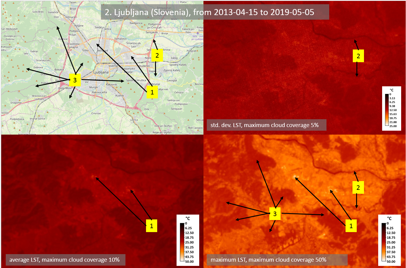 Area of Ljubljana city was analyzed with multi-temporal processing from 15.4.2013 to 5.5.2019. Results are images with standard deviation, average and maximum LST values with 5%, 10% and 50% cloud coverage or less. Average and maximum LST values show for possible urban heat islands in the shopping and business zones of the city (1). Maximum and Standard deviation LST show quite distinctively rivers Sava and Ljubljanica (2). Maximum LST values also point out the vegetation areas in and around the city (3).
- Florida (USA)
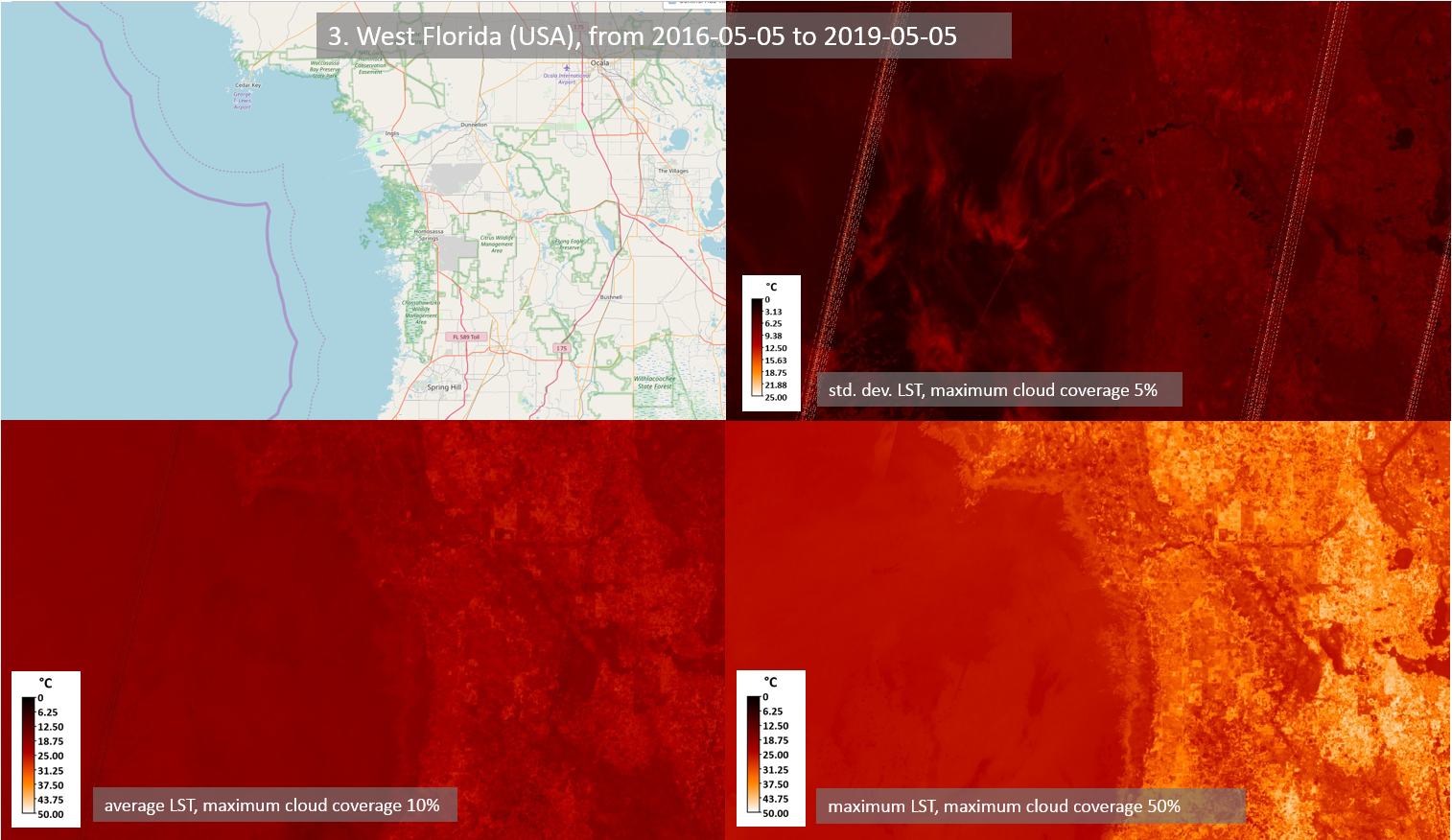 West Florida was analyzed with multi-temporal processing from 23.3.2013 to 5.5.2019. Results are images with Standard deviation, average and maximum LST values with 5%, 10% and 50% cloud coverage or less. Generally, we can distinguish various land covers with maximum LST. On the east, more urban areas are quite visible with high maximum LST values. Rivers, lakes and coastal area with wildlife have lower LST values as expected. Standard deviation values clearly show the influence of clouds on the variation of values. Consequently, it is expected that average LST values were quite influenced by cloud coverage, even though that is not obvious on the image with average LST values. In addition, standard deviation and average LST values are affected by the boundary of the image.
References
Main theory to calculate land surface temperature:
[1] Avdan, U., Kaplan, G. J., 2016. Algorithm for Automated Mapping of Land Surface Temperature Using LANDSAT 8 Satellite Data. Journal of Sensors. 2016. 1-8. 10.1155/2016/1480307.
[2] Orhan, O., Yakar, M., 2016. Investigating Land Surface Temperature Changes Using Landsat Data in Konya, Turkey.
[3] Salih, M. M., Jasim, O. Z., Hassoon, K. I., Abdalkadhum, A. J., 2018. Land Surface Temperature Retrieval from LANDSAT-8 Thermal Infrared Sensor Data and Validation with Infrared Thermometer Camera.
Other helpful references:
[4] El-Hattab, M., Amany, S. M., Lamia, G.E., 2018. Monitoring and assessment of urban heat islands over the Southern region of Cairo Governorate, Egypt.
[5] Franzpc, 2018. How to calculate Land Surface Temperature with Landsat 8 satellite images. GeoGeek by franzpc.
[6] Mehebud, S., Raihan, A., Haroon, S., 2016. Analyzing land surface temperature distribution in response to land use/land cover change using split window algorithm and spectral radiance model in Sundarban Biosphere Reserve, India.
[7] ResearchGate, 2015. NDVI value to extract bare soil pixels for Landsat TM.
[8] Saleh, A. M., 2018. Land Surface Temperature Retrieval of Landsat-8 Data Using Split Window Algorithm-A Case Study of Mosul District. College of Agriculture /University of Baghdad.
[9] Sentinel-Hub Forum, 2018. Landsat Thermal.
[10] UW-Madison, 2019. Vegetation Index NDVI. Satellite Meteorlogy, University of Wisconsin-Madison.
[11] Xiaolei, Y., Xulin G., Zhaocong W., 2014. Land Surface Temperature Retrieval from Landsat 8 TIRSóComparison between Radiative Transfer Equation-Based Method, Split Window Algorithm and Single Channel Method. Department of Geography and Planning, University of Saskatchewan; School of Remote Sensing and Information Engineering.