Visualising floods using Sentinel-1 overlaid on Sentinel-2 imagery
//VERSION=3
function setup() {
  return {
    input: [{
        datasource: "S2L2A",
        bands: ["B08", "B03", "B04", "CLM", "CLP"]
      },
      {
        datasource: "S1GRD",
        bands: ["VV", "VH", "dataMask"]
      }
    ],
    output: { bands: 4 },
    mosaicking: "SIMPLE"
  };
}

function toDB(input){
  return 10 * Math.log(input)/Math.LN10;
}

function evaluatePixel(sample) {
  var S1 = sample.S1GRD[0];
  var S2 = sample.S2L2A[0];
  if (toDB(S1.VV) <= -15){
    return [S1.VV * 10, S1.VV * 10 , S1.VV * 50, 1];
  } else {
    const f = 2.5;
    return [f*S2.B08,f*S2.B08, f*S2.B08,1]
  }
}
//VERSION=3
function setup() {
return {
input: [
{
datasource: "S2L2A",
bands: ["B08"],
},
{
datasource: "S1GRD",
bands: ["VV", "dataMask"],
},
],
output: { bands: 4 },
mosaicking: "SIMPLE",
};
}
function toDB(input) {
return (10 * Math.log(input)) / Math.LN10;
}
//threshold value for water detection, reduce for more water, increase for less water
const lim = 15;
//gain value for image brightness (increase for brighter image)
const f = 2.5;
function evaluatePixel(sample) {
var S1 = sample.S1GRD[0];
var S2 = sample.S2L2A[0];
if (toDB(S1.VV) <= -1 * lim) {
return [S1.VV * 10, S1.VV * 10, S1.VV * 50, 1];
} else {
return [f * S2.B08, f * S2.B08, f * S2.B08, 1];
}
}//VERSION=3
function setup() {
return {
input: [
{
datasource: "CUSTOM",
bands: ["B02", "B03", "B04"],
},
{
datasource: "S1GRD",
bands: ["VV", "VH", "dataMask"],
},
],
output: { bands: 4 },
mosaicking: "SIMPLE",
};
}
function toDB(input) {
return (10 * Math.log(input)) / Math.LN10;
}
//threshold value for water detection, reduce for more water, increase for less water
const lim = 15;
//gain value for image brightness (increase for brighter image)
const f = 0.0008;
function evaluatePixel(sample) {
var S1 = sample.S1GRD[0];
var S2 = sample.CUSTOM[0];
if (toDB(S1.VV) <= -1 * lim) {
return [S1.VV * 10, S1.VV * 10, S1.VV * 50, 1];
} else {
return [f * S2.B04, f * S2.B03, f * S2.B02, 1];
}
}Evaluate and Visualize
Authors
Author of the datafusion script:
- William Ray & Maxim Lamare
Evaluate and visualize
General description of the script
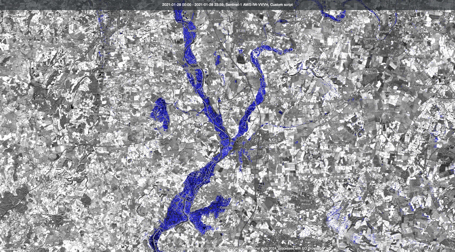
This script can be used to visualise flood events using Sentinel-1 GRD imagery. This is especially useful for areas of interest that are affected by cloud cover (common during flood events caused by excessive rainfall). The script uses a threshold of -15 decibels to classify flooded pixels. This value can be adjusted to suit your area of interest using the lim parameter. In addition, to help the viewer orientate themselves, a clear Sentinel-2 image is used as the basemap for this visualisation so that it can be easily interpreted where the flood extent reaches for those unfamiliar with interpreting SAR images.
How to use
- Select your area of interest
- From Data Collections, select
Sentinel-2 MosaicorSentinel-2 L2A. You can choose the most recent mosaic or the one from the same season as your time of interest; if you are selecting a single image, make sure it is cloud free. - From Layers, select Custom Script. Click the Custom Script tab, and check the
Use additional datasets (advanced)box. UnderAdditional datasets, you will seeS-1 GRD. Click the+Sign to add it. Make sure you enable orthorectification. Optionally, you can also use a speckle filter. - Check the
Customize timespanbox and select the timeframe you are interested in (the timeframe of your flood) - Now paste the script in the code field. Take care to use the right one,
Copernicus Browserif you are using a single Sentinel-2 image as a background andSentinel-2 Mosaicif you want the mosaic background. Then clickRefresh Evalscript. - If you want to adjust the brightness of the background image, change the
fconstant. It is typically around 2.5 for Sentinel-2 images and 0.0008 for Sentinel-2 mosaics, increasing the gain makes the image brighter.
Interpretation of results
Flooded areas will be marked in blue. Since this is a SAR dataset, the resulting map is affected by SAR speckle. In some cases, wet vegetation fields, steep slopes facing away from the sensor, or large flat surfaces such as airports can also create low backscatter and can thus be mistaken for flooded areas. Therefore, the 3D view can also be helpful for interpreting results: flooded areas are usually in the valley bottoms.
Verification of flooding on a 3D image 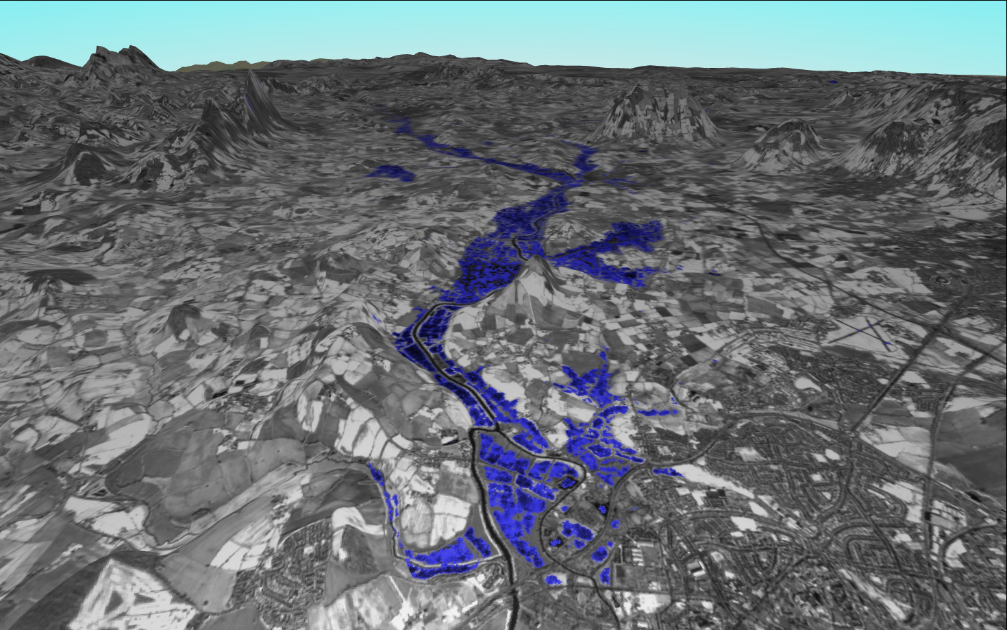
Description of representative images
In late 2023 and early 2024, north-western Europe experienced very high levels of rainfall, which led to widespread river flooding. This scene shows the Severn River upstream of Gloucester on 01 January 2024, with a Sentinel-2 image from 28 February 2024 as a background.
Flooding in the UK 28th January 2021